Hello World & Installing Python and Jupyter
Like many social scientists I was taught very little programming in grad school. I knew how to point and click my way through SPSS and I knew how to to do some "proc reg" commands in SAS. That was about it. As I started to deal with more and more data in SPSS and Excel I started to realize there were tons of redundancies and a lot of my time was spent recreating very similar analyses to answer slightly different questions.
At the same time I started to see many "Machine Learning Experts" creep into the I/O & Selection Space saying they could leverage ML to predict the perfect employee.
I thought we were trying to solve the same problem, they can't be doing things that differently than us, so I started to dive into basic ML literature. My first experience with ML was this book and I started to see that ML wasn't that different than many of the things social scientists were traditionally trained to do, they just used different terminology, which made it seem foreign to us.
My hope for this blog is it can be something that helps Social Scientists interested in adding programming and data analysis to their core skillset get that knowledge in a way that made sense for someone coming from their background.
print('Hello World!!')

Starting with the basics
One thing that has always been fairly cumbersome is setting up your working environment in python. In SPSS you pay for the software, you install it and you are good to go. You want to run a correlation. There's a dropdown in the menu for that. A linear regression, a drop down in the menu for that. The difference between SPSS and Python is that SPSS is a ready to use software solution designed with a specific purpose. On the other hand Python is a general use programming language. Do you want to build a website? The flask and django packages can help with that. Do you want to perform math? Basic Python has you covered there. More advanced linear algebra? NumPy's broadcasting has you covered. For this reason your environment is important. You would use a different environment to build a website than you would to perform a statistical analysis. This is where the specific packages come in. One place where most packages are compiled and kept up-to-date is Anaconda. Anaconda is a distribution of the most common packages used for data science and machine learning.
In this first post I will walk you through the process of downloading Anaconda and setting up your first Data Science Environment
Step:
- Download and install Anaconda or Miniconda
- This site will give you the installation for your specific OS.
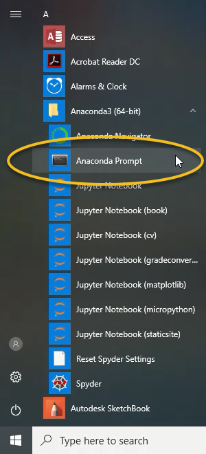
- If you are in Windows in your start menu after installation you should be able to search for Anaconda Prompt.
- If you are in Linux or Mac you can use the actual terminal.
- This site will give you the installation for your specific OS.
Open Anaconda Prompt or the terminal and you should see something similar to the image below
After successfully installing Anaconda you can use conda commands.
- This is where you will create your first virtual environment. A virtual environment is extremely important when it comes to keeping your work environment from being overrun by packages (collections of python files) you aren't using for your specific project. You can then specify the version of python you want. I want my environment to be in python 3.7, so I will specify that in the creation by writing the following:

-n stands for (name) so after the -n command you will name your virtual environment. For the purposes of this example I named mine my_first_venv and specified the python version to be 3.7.
There are differences between Python 2 and Python 3, that are beyond the scope of this blog, but most new data analysis and data science methods will be more routinely updated in python 3.
In fact Guido van Rossum, the creator of Python has told the community Python 2 will stop being support in January of 2020. You can view the countdown here.
Getting into our virtual environment
Now that we have built our virtual environment let's use it. You can do that by using the source activate command and the name of the virtual environment you created above. Similar to what I did below.
Note When you are finished in your virtual environment you just use the command source deactivate and you will be back to a normal bash shell/terminal.
You successfully navigated into your first virtual environment. Now anything you run or do will be working strictly off of the packages in this virtual environment.
Next you can install the common packages that you'll need for data analysis/data science, here are a few:
- conda install numpy
- numpy is a linear algebra library, which pandas is built on top of
- conda install pandas
- pandas) is a dataframe library (structures data similar to excel)
- conda install scikit-learn
- scikit learn is a machine learning library
- conda install -c conda-forge matplotlib
- matplotlib is a visualization library
- conda install -c anaconda seaborn
- seaborn is an advanced visualization library built on top of matplotlib
Downloading Jupyter and Creating a Jupyter Kernel
Most people running data analyis won't want to work in a traditional developers IDE (Integrated Development Environment), like PyCharm because it's fairly cumbersome to debug code when you can't run it in line. For this reason I think Jupyter is an excellent solution for people that are unlikely to be productionizing their analysis, but instead will be trying to derive quick calculations, like means, standard deviations, correlations, etc.
Jupyter stands for 3 programming languages:
and allows you to develop and test code within your web browser which is extremely convenient for quickly prototyping analyses or simple functions.
So let's create a kernel specific to our virtual environment, so we can use jupyter in our browser.
First thing we need to do is install ipykernel in our virtual environment.

Next we activate the notebook by typing the following command:

If that doesn't launch the notebook in a browser you can use the following command in your terminal/anaconda prompt

Note I don't typically work in Windows or MacOS, but I have been told that once Jupyter is installed on your computer you can also just launch it by searching through the START menu. If that's the case I'd recommend creating a shortcut on your desktop, so you can just double-click and get it started. It might look like below, where the anaconda prompt is circled and immediately below it is the jupyter notebook application.
This will launch a web browser that allows you to interact with your directories. You can navigate through your directories to where you plan to work on your project. You can do this through the browser.
Over on the far right of the web browser you will see a tab titled New. You can see here that I have a few virtual environments with kernels, from an R kernel to many different kernels for different projects.
You will click on my_first_venv and it will open up a jupyter notebook with that kernel.

Once you click on my_first_venv you will get a notebook that pops up and looks identical to this:

Now that you are in the notebook you can start your work. Here is an example of some basic math operations happening in line. In a python script you'd typically need to call the print command to see the output.
Basic Math
4+4
35*5
print ("Let's learn some python!!")
In follow up posts I'll start to talk about using numpy and pandas and their importance to data science and the value I think they can add for your typical Social Scientists.
